From Zero to a Working YOLO Classifier on Oracle Cloud: Training an Insect Model End-to-End with OCI Data Science + Object Storage + Gradio

There’s a very practical question behind many AI conversations with customers:

“Do we actually have the infrastructure to run and iterate on computer vision models reliably?”

This project started as a hands-on way to answer that question with a concrete artifact:
a working YOLO-based image classification model, trained on a real dataset, packaged with a Gradio demo. All running on Oracle Cloud Infrastructure (OCI), with OCI Data Science as the core development environment.

The result is an end-to-end reference implementation you can reuse not only for insect classification, but for any multi-class image classification scenario (quality checks, defects, product categories, document types, plants, animals… you name it).

What I built in high level

I implemented a complete workflow:

1. Connect to OCI Object Storage using Resource Principals (no secrets in notebooks).
2. Prepare a dataset split (train/ + val/), organized by class folders.
3. Run dataset QA + EDA (class distribution, sample grids, image sizes, sanity checks).
4. Train a YOLOv8 classifier (Ultralytics) on a CPU instance in OCI Data Science.
5. Evaluate metrics and latency, export artifacts (including ONNX).
6. Deploy a simple Gradio app to upload an image and get predictions.

Compute used: OCI Data Science notebook session on VM.Standard.E5.Flex (4 OCPU)
Training time: ~3 hours for 30 epochs on the Kaggle insect dataset.

That’s already strong proof that the baseline infrastructure works. And it’s also the perfect starting point to discuss scaling:

• more OCPUs / RAM for faster CPU training
• GPU shapes for heavy training or larger models
• productionization with pipelines, model deployments, and governance

Use case: insect classification as a starter for real customer problems

We used an insect dataset because it’s a clean, public benchmark-like example: it has multiple classes, real variation, and enough images to stress the workflow.

But the pattern matters more than the subject.

This same pipeline maps cleanly to customer scenarios such as:

• Defect classification for manufacturing quality (surface issues, cracks, corrosion)
• Visual categorization for retail / e-commerce
• Asset inspection (infrastructure, equipment, drones)
• Document image types (forms, IDs, invoices, stamps)
• Biodiversity monitoring (species classification, invasive detection)

This project is designed as a blueprint: a functional codebase from ingestion → training → evaluation → demo.

What is YOLO? And why use it for classification?

YOLO stands for “You Only Look Once”, a family of deep learning models known historically for real-time object detection. Modern YOLO ecosystems (like Ultralytics YOLOv8) also support:

• classification
• detection
• segmentation
• pose

For this project we used YOLOv8 Classification, which gives you:

• lightweight and production-friendly architectures (e.g., yolov8n)
• strong tooling (training logs, metrics, exports)
• portability via standard formats (PyTorch weights, ONNX export, etc.)

What is OCI Data Science?

OCI Data Science is Oracle’s managed service for building, training, and deploying ML models on OCI. In practice, it gives you:

• Notebook Sessions (your development runtime in the cloud)
• Jobs (run training/ETL at scale and on schedule)
• Model Catalog & Deployments (go from trained model → endpoint)
• Integration with OCI services (IAM, Object Storage, Logging, Monitoring)

It’s the “workbench” that made this whole workflow consistent:

• reproducible environment (no “it works on my laptop”)
• secure access to data in Object Storage
• flexible compute for experiments and scaling

CPUs vs GPUs in OCI Data Science

OCI Data Science lets you pick compute shapes depending on your workload:

CPU shapes. Great for:

• fast prototyping and data prep
• classical ML / lighter DL training
• inference benchmarking
• smaller CV models or limited datasets

In this project, we used VM.Standard.E5.Flex (4 OCPU) and completed 30 epochs in ~3 hours.

GPU shapes. Great for:

• deep learning training at scale
• larger models / higher-resolution images
• faster iteration cycles (more experiments per day)

If a customer needs faster training or heavier experimentation, GPUs are the natural next step. The key is matching the shape (VRAM, GPU count) to:

• model size
• batch size
• image resolution
• augmentation complexity

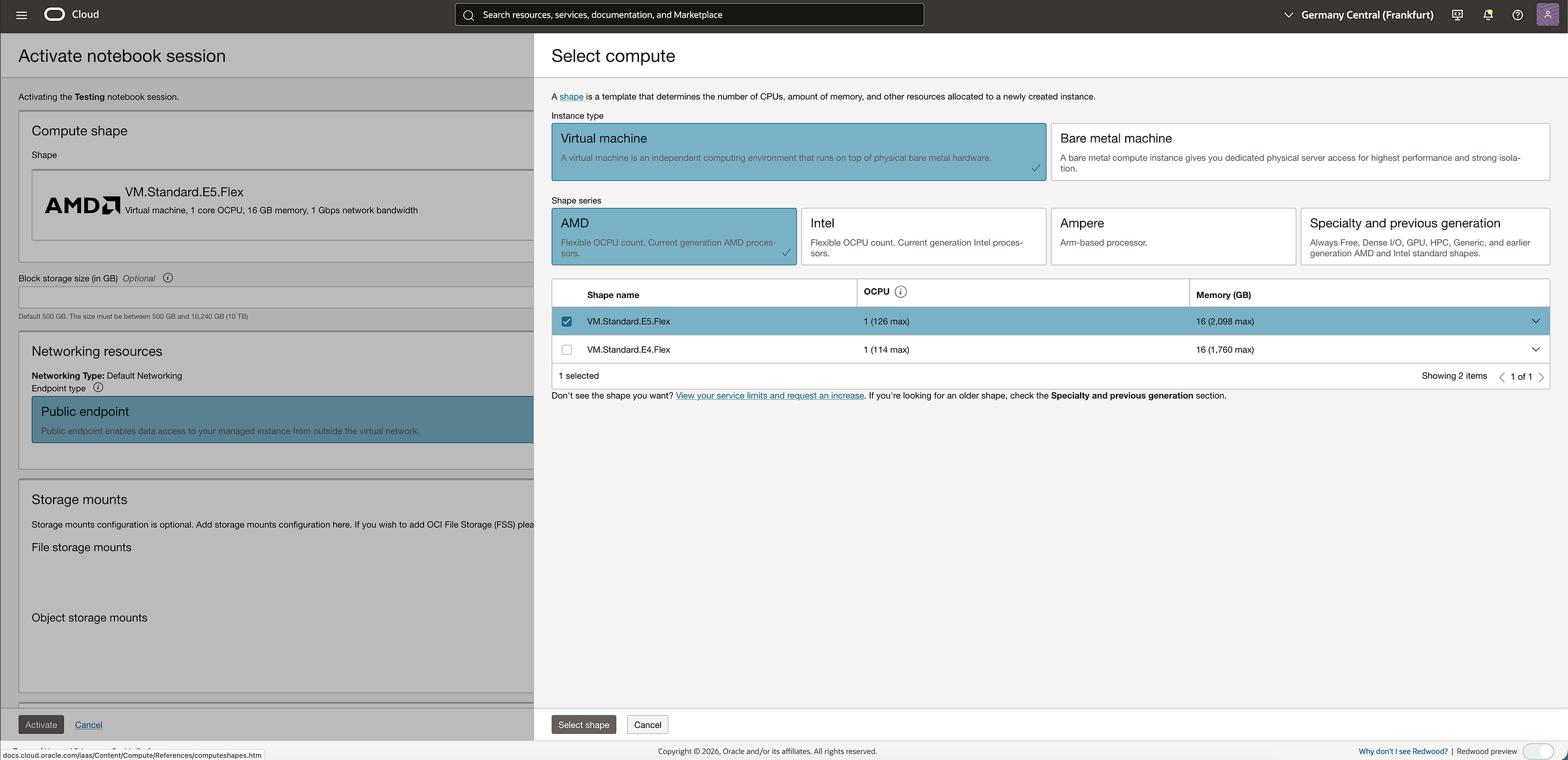
Check here the available CPU/GPU shapes: https://docs.oracle.com/en-us/iaas/Content/Compute/References/computeshapes.htm

And if you want to deeply understand which shape is the best for your use case, check this article I wrote recently! : Choosing the right GPU shape in OCI Data Science for your AI Model: A practical guide

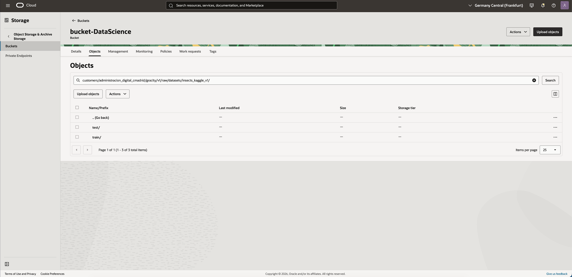
OCI Object Storage: where the data and artifacts live

OCI Object Storage is the standard place to store:

• training datasets (train/, val/), versioned by prefix
• model outputs (runs/…)
• exported models (best.pt, best.onnx)
• logs and metrics

It’s durable, scalable, and integrates cleanly with OCI IAM policies.

---

How we securely connect to Object Storage (Resource Principals)

Rather than embedding API keys, we used Resource Principals.

Conceptually:

• the notebook session (a cloud resource) gets an identity
• IAM policies grant it access to specific buckets/prefixes
• the notebook authenticates automatically via the resource’s identity

In code:

• create signer via oci.auth.signers.get_resource_principals_signer()
• instantiate ObjectStorageClient(config={}, signer=signer)
• read namespace and list/upload objects

This is a best practice for customer-facing work because it keeps credentials out of code and reduces operational risk.

---

Step-by-step: what the code does (00 → 06) — code-level narrative

Below I’m describing what each notebook actually implements, at the level of functions/variables and the main “execution path”, so the reader understands the mechanics (not just the intent). 

You can access to the whole project here: https://github.com/Cristina-Varas/oci-yolov8-image-classification/tree/main

00 — Environment + OCI Access (00_environment_oci_access.ipynb)

Goal: prove the notebook runtime can authenticate to OCI and reach Object Storage without secrets.

Key things in code

Uses Resource Principals:

• signer = oci.auth.signers.get_resource_principals_signer()
• os_client = ObjectStorageClient(config={}, signer=signer)

Fetches the Object Storage namespace (required for most calls):

• namespace = os_client.get_namespace().data

Validates access by listing objects under a prefix:

• os_client.list_objects(namespace, BUCKET_NAME, prefix=DATASET_PREFIX)

This is the security baseline: if this works, you can read/write datasets + artifacts from any notebook/job in that compartment, driven by IAM policies.

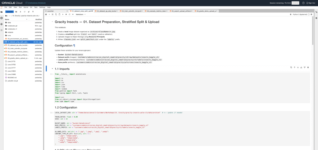
01 — Dataset preparation (split + upload) (01_dataset_prep_split_upload.ipynb)

Goal: build a clean ImageNet-style folder dataset and upload it to Object Storage with a predictable structure.

What the code does

1. Dataset root conventions

• Defines local paths like:
• RAW_ROOT: Path (where the raw images land locally)
• OUT_ROOT: Path (prepared output)
• TRAIN_DIR = OUT_ROOT / "train"
• VAL_DIR = OUT_ROOT / "test" (or val/ if you rename; YOLO expects train/ + val/)

1. Split logic

Iterates per class folder, collects image file paths, shuffles with a fixed seed:

• random.Random(SEED).shuffle(items)

Splits according to ratios (e.g., 80/20):

• n_val = int(len(items) * VAL_RATIO)

Copies or symlinks images to:

• train/<class>/...
• test/<class>/... (starter shortcut)

2. Upload to Object Storage

Uses put_object(...) per file:

• object_name = f"{DATASET_PREFIX}/train/{cls}/{filename}"
• os_client.put_object(namespace, BUCKET_NAME, object_name, put_object_body=f.read(), ...)

Optionally prints progress counts for traceability.

Ultralytics classification reads folder datasets directly. A consistent layout avoids 90% of “silent dataset bugs”.

02 — Dataset QA & EDA (02_dataset_qa_eda_bucket_first_fixed.ipynb)

Goal: sanity-check that what you uploaded is correct, balanced enough, and visually consistent.

What the code does

1. Sync a small subset locally (bucket-first)

Lists objects in the bucket for train/ and test/

Downloads only what you need (either full dataset or subset) into:

• LOCAL_ROOT / train/...
• LOCAL_ROOT / test/...

2. Counts per class

Walks folders and counts image files:

• returns a dict: {class_name: count}

Creates a pandas.DataFrame for easy viewing + sorting.

3. Random visual inspection grid

Picks a few random samples per class.

Reads with cv2 and converts BGR→RGB:

img = cv2.cvtColor(cv2.imread(str(p)), cv2.COLOR_BGR2RGB)

• Displays with matplotlib in a grid.

4. Image size distribution

For a sample of images, reads shapes:

• h, w = img.shape[:2]

Plots histograms / basic stats to catch:

• huge outliers
• tiny thumbnails
• inconsistent aspect ratios

It’s the checkpoint before training. If you see incorrect labels, duplicates, or weird resolutions here, you fix it before wasting compute.

03 — Training (YOLOv8 classification) (03_train_yolov8n_cls.ipynb)

Goal: train a YOLOv8 classifier and produce reproducible run artifacts.

What the code does

1. Ensure dataset is in the format YOLO expects

Ultralytics classification expects:

• dataset_root/train/...
• dataset_root/val/...

If your bucket uses test/, the notebook creates a local alias:

• val_alias = dataset_root / "val"
• val_alias.symlink_to(test_dir, target_is_directory=True)

2. Training config

Central hyperparameters:

• MODEL_NAME = "yolov8n-cls.pt"
• IMGSZ, EPOCHS, BATCH
• DEVICE = "cpu" (important if no CUDA)
• SEED and RUN_NAME for reproducibility

3. Train call

Loads model:

• model = YOLO(MODEL_NAME)

Runs training:

• results = model.train(data=str(dataset_root), imgsz=IMGSZ, epochs=EPOCHS, batch=BATCH, device=DEVICE, project=PROJECT_DIR, name=RUN_NAME, seed=SEED)

Writes artifacts to:

• runs/<RUN_NAME>/...
• runs/<RUN_NAME>/results.csv
• runs/<RUN_NAME>/weights/best.pt, last.pt

4. Quick run verification

Opens results.csv as a DataFrame and prints tail/head.

Optionally plots metrics/accuracy_top1 over epoch.

This produces the “training evidence”: metrics + weights + configs, which you can version, compare, and later deploy.

04 — Evaluation + latency (04_evaluate_metrics_latency.ipynb)

Goal: evaluate the model beyond the training log and measure inference time on CPU (E5 Flex in this case).

What the code does

1. Load the trained weights

Uses the actual file:

• WEIGHTS_PATH = RUN_DIR / "weights" / "best.pt"
• model = YOLO(str(WEIGHTS_PATH))

2. Build a validation list

Iterates val/<class>/image.jpg and stores:

• val_items: List[Tuple[Path, str]] = [(img_path, class_name), ...]

3. Run predictions and compute accuracy

For each image:

• out = model.predict(str(img_path), verbose=False, device="cpu")
• probs = out[0].probs
• pred = model.names[int(probs.top1)]

Computes:

• overall accuracy
• optional per-class confusion matrix (if included)

4. Latency benchmarking

Warms up model with one inference.

Times N inferences:

• t0 = time.perf_counter(); ...; dt = time.perf_counter() - t0

Reports:

• avg latency / image
• p50 / p95 if you compute percentiles

Customers often ask: “How fast is it?” Latency gives you a baseline for sizing (CPU vs GPU, replicas, concurrency).

05 — Export + upload artifacts (05_export_upload_artifacts.ipynb)

Goal: make deployment-ready artifacts and push them back to Object Storage for traceability.

What the code does

1. Resolve run paths

• RUN_PATH = Path("runs/.../<RUN_NAME>")
• BEST_PT = RUN_PATH / "weights" / "best.pt"

2. Export to ONNX

• model = YOLO(str(BEST_PT))
• onnx_path = model.export(format="onnx", opset=17, dynamic=False)

Produces:

• best.onnx in the weights directory

3. Upload artifacts folder

Defines:

• RUNS_PREFIX in the bucket (e.g., .../runs/...)

Upload function walks the directory recursively and does put_object for each file.

Stores artifacts under:

• <RUNS_PREFIX>/<RUN_NAME>/...

This is your reproducibility + governance layer: training artifacts stored centrally, not “lost” inside a notebook VM.

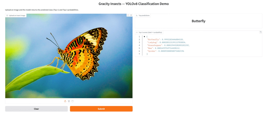
06 — Gradio demo (06_gradio_demo_upload_predict.ipynb)

Goal: provide a simple UI for stakeholders: upload an image → get prediction (Top-1 + Top-K).

What the code does

1. Load model once

• MODEL_PATH = Path(.../"best.pt") (or ONNX if you prefer)
• model = YOLO(str(MODEL_PATH))

2. Prediction function

Accepts a PIL.Image from Gradio.

Converts to RGB and saves to a temp file (Ultralytics likes file paths):

• tmp_path = ...; image.save(tmp_path)

Calls:

• pred = model.predict(str(tmp_path), verbose=False, device="cpu")[0]

Extracts probabilities:

• probs = pred.probs
• topk_idx = probs.top5

Builds {label: float(prob)}

3. Gradio Interface

Input:

• gr.Image(type="pil")

Outputs:

• gr.Label(num_top_classes=5) (nice UI for Top-K)
• gr.JSON() (raw dict with scores)

Launch:

• demo.launch(server_name="0.0.0.0", server_port=7860, share=False) (or share=True if allowed)

It converts an ML notebook into a “demoable product” immediately. Perfect for customer meetings and for validating real images.

Mini note on preprocessing

For YOLOv8 classification, preprocessing is mostly handled internally:

• resizing to imgsz
• normalization
• augmentations during training (if enabled)

What is worth adding (if the customer’s real images differ from Kaggle):

• optional resizing/compression during upload to reduce storage/transfer
• standardization (e.g., enforce JPEG quality, max dimension)
• background/lighting augmentation if production images vary strongly

High accuracy early is usually a good sign, but always validate:

• class balance (no underrepresented classes being ignored)
• label quality (folder names match true labels)
• data leakage risk (duplicates between train and test/val)
• real-world representativeness (lighting, camera types, background variation)

Where this goes next: production on OCI (ADB + APEX)

A prototype becomes a product when we introduce governed data, repeatable pipelines, and a UI.

Oracle provides a clean end-to-end path:

• store labels/predictions/metadata in Autonomous Database
• orchestrate retraining with OCI Data Science Jobs
• deploy the model through OCI Data Science Model Deployment
• build a user-facing app in Oracle APEX:
• image upload
• prediction display
• review + relabel (human-in-the-loop)
• monitoring dashboards

So this insect classifier isn’t “just a demo”. It’s a repeatable architecture pattern.

Links & resources

• Notebooks / full code on GitHub: https://github.com/Cristina-Varas/oci-yolov8-image-classification/tree/main
• LinkedIn: https://www.linkedin.com/in/cristina-varas-menadas-591825119/
• Website: cristinavaras.com 

Cristina Varas Menadas — Data Scientist