From Lat/Lon to Hexagons and Neighbourhoods: Learning H3 with Madrid

How a bird-sighting anomaly project turned into a reusable H3 geospatial demo.

When you work with geospatial data, you quickly run into this question:

I have latitude and longitude… now what?

This article is a practical walk-through of a Jupyter notebook that answers exactly that, using H3 and Madrid as a playground.

The notebook originally came from a real customer project on bird-sighting anomaly detection, where we had almost nothing but coordinates. I kept exploring the idea and turned it into a clean, reusable demo you can plug into your own workflows.

Disclaimer: This is a personal project and is not affiliated with, endorsed by, or representing Oracle in any way. All opinions and content are my own.

1. The story: bird sightings, poor data, and the “where” problem

This whole project started with a real customer use case.

We were building an anomaly detection model for bird sightings. The goal was to detect suspicious observations — birds reported in locations where they typically shouldn’t appear.

The problem? The dataset was extremely poor.

For each sighting we had:

• A timestamp
• A species identifier
• A latitude and longitude

We did not have:

• Country
• Region
• City
• Neighbourhood
• Any higher-level geographic labels

If you want to model “unusual locations” but all you have is 40.4168 and -3.7038, you’re missing a crucial layer of meaning. We needed a way to turn continuous coordinates into discrete, interpretable locations.

My first idea was the obvious one:

Let’s call a geocoding API and ask for the barrio, or even the street, of every point.

That works if you have a few hundred points. But when you have hundreds of thousands of rows, the story changes:

• You need one API call per coordinate.
• You’ll hit rate limits very quickly.
• The estimated runtime for our dataset was on the order of 600 hours (yes, days or months of geocoding).

So I needed another solution: something local, fast, and friendly to analytics and ML.

That’s when H3, Uber’s hexagonal hierarchical geospatial index, became the core building block.

This article is a cleaned-up, reusable version of that work. I turned it into:

• A Jupyter notebook, and
• A small GitHub project

that you can plug into your own workflows to go from:

lat, lon → H3 hexagon → neighbourhood → features & visualisations

We’ll use synthetic data over Spain and then zoom into Madrid as a concrete example.

2. What is H3, really?

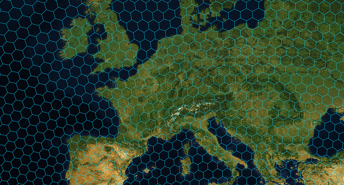
H3 is an open-source geospatial indexing system originally developed at Uber.

At a high level:

It divides the Earth’s surface into hexagonal cells (plus a few pentagons).

Each cell gets a unique H3 index (a string).

It supports resolutions from 0 to 15:

• Low resolution (0–3): huge cells, continent or country scale.
• Medium (5–7): region / city / neighbourhood scale.
• High (10+): street / building scale.

It is hierarchical:

• A cell at resolution r is subdivided into several children at resolution r+1.
• You can “zoom in” or “zoom out” programmatically.

Why is this useful?

Because instead of thinking:

This sighting occurred at (40.4168, -3.7038)

we can think:

This sighting occurred in H3 cell 87390c2a7ffffff at resolution 7,
which happens to be inside the Ventas neighbourhood in Madrid.

That makes it much easier to:

• Aggregate data (counts per cell)
• Compare locations (neighbouring cells)
• Build features for ML models (cell-level statistics)
• Visualise patterns (hexagonal heatmaps)

In this article, we’ll use H3 to:

1. Index synthetic points across Spain

2. Zoom into Madrid

3. Attach barrios and distritos using official city polygons

4. Visualise everything as both:

• A choropleth by neighbourhood, and
• A hexagonal heatmap by H3 cell

3. The GitHub notebook behind this article

All the code in this article lives in a small GitHub project with a structure like:

h3-madrid-demo/
├─ notebooks/
│ ├─ 01_h3_spain_madrid_demo.ipynb
├─ data/
│ ├─ raw/
│ │ ├─ spain_h3_demo_points.csv # synthetic Spain points
│ │ ├─ BARRIOS.* # Madrid neighbourhood shapefile
│ └─ processed/
│ ├─ spain_h3_demo_points_enriched.csv
│ └─ madrid_h3_points_with_barrios.csv
├─ figures/
│ ├─ fig01_scatter_spain.png
│ ├─ fig02_madrid_barrio_heatmap.png
│ └─ fig03_madrid_h3_hex_heatmap.png
├─ env/
│ └─ environment.yml
├─ src/
│ ├─ h3_utils.py # optional helper functions
├─ README.md
└─ LICENSE

In this article I’ll focus on the notebook and the ideas behind each step.
If you want to run it locally, you’ll find installation and usage details in the README of the repo.

4. Data and basic setup

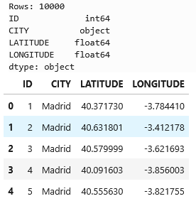
The notebook uses a small synthetic dataset:

10,000 points around several Spanish cities, including Madrid.

Columns:

• ID
• CITY
• LATITUDE
• LONGITUDE

4.1. Imports

We start with standard imports plus h3 and plotting config:

import pandas as pd
import numpy as np
import matplotlib.pyplot as plt

from pathlib import Path

try:
    from h3 import h3  # common pattern
except ImportError:
    import h3          # fallback

%matplotlib inline
plt.rcParams["figure.figsize"] = (8, 6)
plt.rcParams["axes.grid"] = True

4.2. Load the synthetic Spain dataset

file_path = Path("data/raw/spain_h3_demo_points.csv")
df = pd.read_csv(file_path)

print(f"Rows: {len(df)}")
print(df.dtypes)
df.head()

At this point you just confirm that:

• The file exists,
• The columns have the expected types.

4.3. A first scatter plot (sanity check)

Before indexing anything, the notebook plots a quick scatter of all points:

fig, ax = plt.subplots()

ax.scatter(
    df["LONGITUDE"],
    df["LATITUDE"],
    s=5,
    alpha=0.4,
)

ax.set_xlabel("Longitude")
ax.set_ylabel("Latitude")
ax.set_title("Synthetic Spain Points – Quick Scatter Plot");

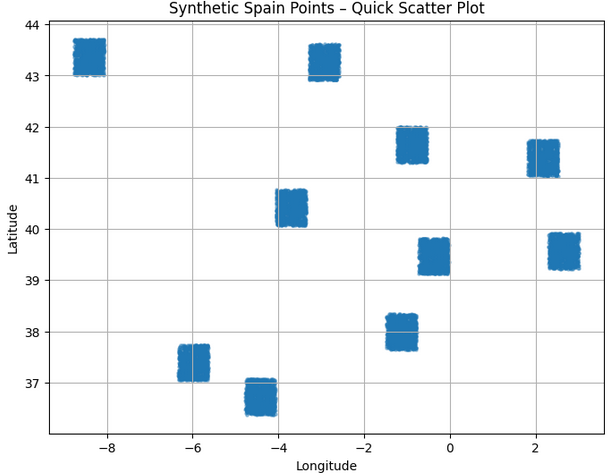
This answers: “Do my points roughly sit on top of Spain? Did I swap latitude and longitude?”

5. Choosing H3 resolutions

We define a set of resolutions to experiment with:

H3_RESOLUTIONS = [5, 6, 7]

Intuition:

• Resolution 5 → big hexagons, good for a Spain-wide view.
• 6–7 → smaller hexagons, good for within-city structure.

In real projects you pick the resolution based on:

• Scale of your analysis (country vs city vs street),
• Data density,
• The type of patterns you care about.

6. From (lat, lon) to H3 index (version-safe helper)

Different versions of the h3 Python package expose different functions:

• Classic: h3.geo_to_h3(lat, lon, res)
• Newer (v4): h3.latlng_to_cell(lat, lon, res)

To keep the notebook robust across environments, I wrap them in a single helper:

import h3  # ensure imported

def latlon_to_h3(lat: float, lon: float, res: int) -> str:
    """
    Convert (lat, lon) in decimal degrees to an H3 index at resolution `res`,
    trying to be compatible with different h3-python versions.
    """
    # Old / classic API
    if hasattr(h3, "geo_to_h3"):
        return h3.geo_to_h3(lat, lon, res)
    # Newer API (v4 style)
    if hasattr(h3, "latlng_to_cell"):
        return h3.latlng_to_cell(lat, lon, res)
    # Fallback: some installs use submodule h3.h3
    try:
        from h3 import h3 as h3core
        if hasattr(h3core, "geo_to_h3"):
            return h3core.geo_to_h3(lat, lon, res)
    except Exception:
        pass

    raise AttributeError(
        "Could not find a suitable H3 function for lat/lon → index. "
        f"Available attributes: {dir(h3)}"
    )

This cell is about defensive coding: if someone runs the notebook with a newer h3, it should still work.

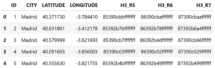
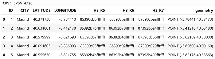
6.1. Applying the helper at multiple resolutions

for res in H3_RESOLUTIONS:
    col_name = f"H3_R{res}"
    df[col_name] = df.apply(
        lambda row: latlon_to_h3(row["LATITUDE"], row["LONGITUDE"], res),
        axis=1
    )
    print(f"Added column: {col_name}")

df.head()

Now each row has:

• H3_R5
• H3_R6
• H3_R7

All points that fall into the same hexagon at resolution 6 will share the same string in H3_R6.

7. How dense is the grid?

To understand the impact of resolution, the notebook counts distinct H3 cells per resolution:

for res in H3_RESOLUTIONS:
    col = f"H3_R{res}"
    nunique = df[col].nunique()
    print(f"Resolution {res}: {nunique} distinct H3 cells")

As res increases:

• The number of cells grows,
• Each cell covers a smaller area,
• Fewer points land in each individual cell.

This gives you intuition to pick a resolution that matches your problem.

8. One point, many resolutions (H3 hierarchy in action)

To make the hierarchy concrete, the notebook takes a single point (preferably in Madrid) and prints its H3 index at several resolutions:

if "Madrid" in df["CITY"].unique():
    sample_row = df[df["CITY"] == "Madrid"].sample(1, random_state=42).iloc[0]
else:
    sample_row = df.sample(1, random_state=42).iloc[0]

lat = sample_row["LATITUDE"]
lon = sample_row["LONGITUDE"]
city = sample_row["CITY"]

print(f"Sample point from city: {city}")
print(f"Latitude:  {lat}")
print(f"Longitude: {lon}\n")

for res in range(3, 9):  # resolutions 3–8
    h3_index = latlon_to_h3(lat, lon, res)
    print(f"Resolution {res}: {h3_index}")

The key idea you want the reader to see:

• The location is the same,
• The H3 index changes with resolution,
• Each index corresponds to a hexagon of a different size, nested within the previous ones.

This is what lets you aggregate at a coarse level and then zoom into finer levels.

9. Zooming into Madrid

So far we’ve treated all Spain the same. For a more concrete story, we focus on Madrid:

df["LATITUDE"] = df["LATITUDE"].astype(float)
df["LONGITUDE"] = df["LONGITUDE"].astype(float)

df_madrid = df[df["CITY"] == "Madrid"].copy()
df_madrid.reset_index(drop=True, inplace=True)

print(f"Total points in original dataset: {len(df)}")
print(f"Points labelled as CITY='Madrid': {len(df_madrid)}")

df_madrid.head()

From now on, the notebook works with df_madrid as the main dataset.

10. Adding neighbourhoods (barrios) via spatial join

H3 gives us a nice grid, but humans think in neighbourhoods, districts, etc.

To add that context we:

1. Load the official “Barrios municipales de Madrid” shapefile (open data).
2. Convert our points to a GeoDataFrame.
3. Use a spatial join to assign each point a:

• BARRIO (neighborhood),
• DISTRITO (district).

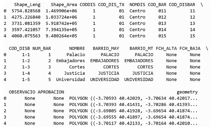
10.1. Load barrios polygons

import geopandas as gpd
from shapely.geometry import Point
from pathlib import Path

barrios_shp_path = Path("data/raw/BARRIOS.shp")

gdf_barrios = gpd.read_file(barrios_shp_path)
gdf_barrios = gdf_barrios.to_crs(epsg=4326)

print(gdf_barrios.head())
print("CRS:", gdf_barrios.crs)

We’ll mainly use:

• COD_BAR – barrio code
• NOMBRE – barrio name
• NOMDIS – district name

10.2. Convert Madrid points to a GeoDataFrame

gdf_points = gpd.GeoDataFrame(
    df_madrid.copy(),
    geometry=gpd.points_from_xy(df_madrid["LONGITUDE"], df_madrid["LATITUDE"]),
    crs="EPSG:4326",
)

10.3. Spatial join: point → barrio and distrito

COD_BAR_COL = "COD_BAR"
BARRIO_NAME_COL = "NOMBRE"
DISTRICT_NAME_COL = "NOMDIS"

gdf_barrios_slim = gdf_barrios[[COD_BAR_COL, BARRIO_NAME_COL, DISTRICT_NAME_COL, "geometry"]].copy()

gdf_joined = gpd.sjoin(
    gdf_points,
    gdf_barrios_slim,
    how="left",
    predicate="within",
)

gdf_joined[[ "CITY", "LATITUDE", "LONGITUDE", "H3_R6", BARRIO_NAME_COL, DISTRICT_NAME_COL ]].head()

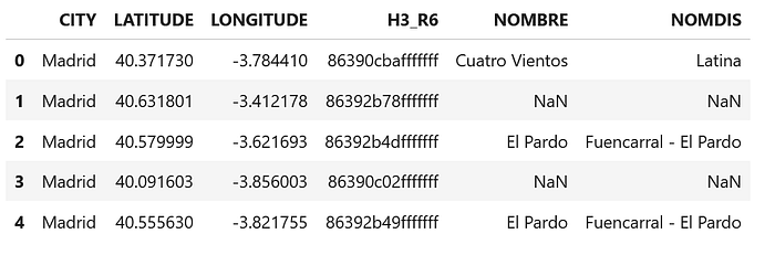
Because our points are synthetic and have some jitter, a few may fall just outside the municipality. For the demo, the notebook simply keeps only points with a valid barrio:

gdf_joined = gdf_joined[gdf_joined[BARRIO_NAME_COL].notna()].copy()
gdf_joined.reset_index(drop=True, inplace=True)

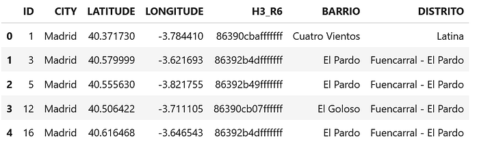
10.4. Clean up and save

gdf_joined.rename(
    columns={
        BARRIO_NAME_COL: "BARRIO",
        DISTRICT_NAME_COL: "DISTRITO"
    },
    inplace=True,
)

df_final = pd.DataFrame(gdf_joined.drop(columns="geometry"))

df_final[["ID", "CITY", "LATITUDE", "LONGITUDE", "H3_R6", "BARRIO", "DISTRITO"]].head()

And save the enriched dataset:

output_final = Path("data/processed/madrid_h3_points_with_barrios.csv")
df_final.to_csv(output_final, index=False)

print(f"✅ Final Madrid dataset with H3 + barrio + distrito saved to: {output_final.resolve()}")

We have now:

• Raw coordinates
• An H3 cell (H3_R6)
• A neighbourhood (BARRIO)
• A district (DISTRITO)

for every point inside Madrid.

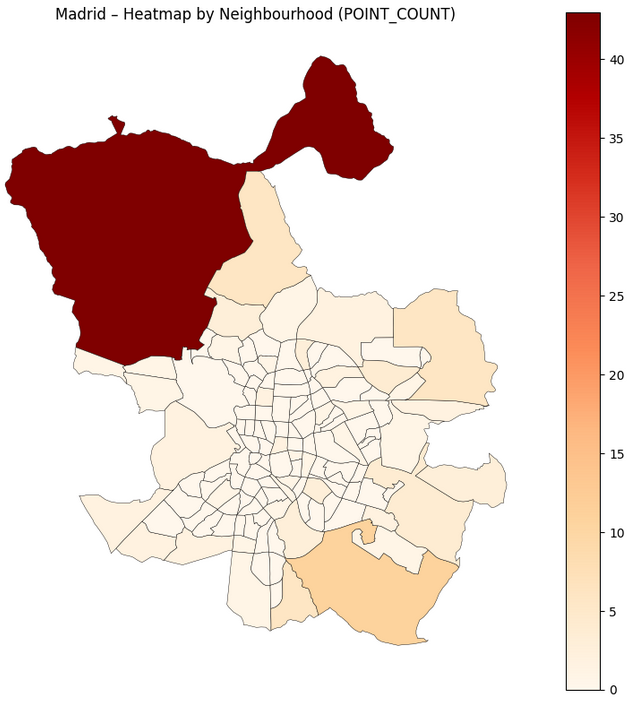
11. Visualisation 1 — Heatmap by neighbourhood

The first visualisation stays in human geography: barrios.

Goal: see which neighbourhoods concentrate more points.

11.1. Aggregate counts per barrio

barrio_counts = (
    df_final
    .groupby("BARRIO")
    .size()
    .reset_index(name="POINT_COUNT")
)

Join with polygons and plot:

barrios_shp_path = Path("data/raw/BARRIOS.shp")
gdf_barrios = gpd.read_file(barrios_shp_path)
gdf_barrios = gdf_barrios.to_crs(epsg=4326)

BARRIO_NAME_COL = "NOMBRE"

gdf_barrios_counts = gdf_barrios.merge(
    barrio_counts,
    left_on=BARRIO_NAME_COL,
    right_on="BARRIO",
    how="left"
)

gdf_barrios_counts["POINT_COUNT"] = gdf_barrios_counts["POINT_COUNT"].fillna(0)

fig, ax = plt.subplots(figsize=(8, 8))

gdf_barrios_counts.plot(
    column="POINT_COUNT",
    ax=ax,
    legend=True,
    cmap="OrRd",
    edgecolor="black",
    linewidth=0.3
)

ax.set_title("Madrid – Heatmap by Neighbourhood (POINT_COUNT)")
ax.set_axis_off()

plt.tight_layout()
plt.show()

12. Visualisation 2 — Hexagonal H3 heatmap

The second visualisation is the H3 view: same data, but aggregated by H3 cell instead of administrative boundaries.

12.1. Build hexagon polygons from H3 indices

from shapely.geometry import Polygon
import h3

def h3_to_boundary(h3_index: str):
    """
    Convert an H3 index to a list of (lat, lon) vertices.
    Compatible with different h3-python versions.
    """
    if hasattr(h3, "h3_to_geo_boundary"):
        return h3.h3_to_geo_boundary(h3_index)
    if hasattr(h3, "cell_to_boundary"):
        return h3.cell_to_boundary(h3_index)
    try:
        from h3 import h3 as h3core
        if hasattr(h3core, "h3_to_geo_boundary"):
            return h3core.geo_to_geo_boundary(h3_index)
    except Exception:
        pass
    raise AttributeError("No suitable H3 boundary function found.")

WORKING_RES = 6
h3_col = f"H3_R{WORKING_RES}"

agg_h3 = (
    df_final
    .groupby(h3_col)
    .size()
    .reset_index(name="POINT_COUNT")
    .rename(columns={h3_col: "H3_INDEX"})
)

polygons = []
for h in agg_h3["H3_INDEX"]:
    boundary = h3_to_boundary(h)
    boundary_lonlat = [(lon, lat) for lat, lon in boundary]
    polygons.append(Polygon(boundary_lonlat))

gdf_hex = gpd.GeoDataFrame(
    agg_h3.copy(),
    geometry=polygons,
    crs="EPSG:4326"
)

12.2. Plot the hex grid

fig, ax = plt.subplots(figsize=(8, 8))

# Optional: barrio outlines for context
gdf_barrios.boundary.plot(ax=ax, color="lightgrey", linewidth=0.5)

gdf_hex.plot(
    column="POINT_COUNT",
    ax=ax,
    legend=True,
    cmap="viridis",
    edgecolor="none",
    alpha=0.8,
)

ax.set_title(f"Madrid – H3 Hexagonal Heatmap (Resolution {WORKING_RES})")
ax.set_axis_off()

plt.tight_layout()
plt.show()

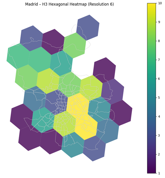
This figure is perfect to explain what H3 does: a regular hexagonal mesh over Madrid, coloured by density.

13. How this generalises to your own data

Even though this came from a bird-sighting anomaly project, nothing in the notebook is specific to birds.

If you have any dataset with coordinates — deliveries, vehicles, IoT sensors, stores, events — you can:

1. Apply the same (lat, lon) → H3 conversion at one or more resolutions.
2. (Optionally) attach administrative context (neighbourhoods, postal codes, regions).
3. Build features per H3 cell:

• Historical counts,
• Ratios vs neighbouring cells,
• Temporal statistics within each cell.

1. Visualise results with hexagonal heatmaps instead of raw points.

The notebook is intentionally simple and linear so you can treat it as a template:

• Replace spain_h3_demo_points.csv with your own CSV.
• Swap the Madrid shapefile for your city or region.
• Adjust a couple of column names.
• Re-run and iterate.

If you build something on top of this — a different city, a new use case, or a more advanced model — I’d love to see it 💙

As always, if you like this content, clap, subscribe to the newsletter, follow me on LinkedIn or check my new website 🙂

Happy coding!